20 Excel Pro Tips for Power Users (With Real-World Examples)

Microsoft Excel remains one of the most versatile business tools in 2025. From budget planning to KPI tracking and executive dashboards, Excel scales from quick ad-hoc analysis to refreshable reporting pipelines. This guide distills 20 field-tested tips I rely on as an IT manager to help teams work faster, reduce errors, and automate repetitive work.

If you’re also modernizing operations with automation and AI, pair this with our practical overview of AI in IT Operations.

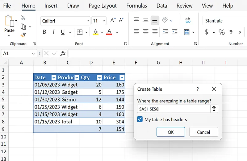
1) Turn Your Data Into a Smart Table

Why: Tables expand automatically, keep formats consistent, and enable readable structured formulas.

Real use: Sales trackers, inventory lists, and project logs stop breaking when rows are added mid-month.

How to do it

1. Select any cell in your range and press Ctrl+T.
2. Check My table has headers if applicable → click OK.
3. Go to Table Design → change Table Name to something meaningful (e.g., SalesTbl).
4. Use structured references in formulas, e.g., =[@Qty]*[@Price].

2) Replace VLOOKUP With XLOOKUP

Why: XLOOKUP searches left/right and handles missing values gracefully; no more brittle column-index math.

Formula: =XLOOKUP(A2, Products[SKU], Products[Price], "Not found")

How to do it

1. Ensure your source is a table (e.g., Products with [SKU] and [Price]).
2. In the result cell, enter =XLOOKUP(lookup_value, lookup_array, return_array, [if_not_found]).
3. Use optional arguments like match_mode (exact/wildcards) when needed.

Learn more on Microsoft’s docs: XLOOKUP.

3) FILTER + SORT + UNIQUE for Instant Reports

Dynamic arrays can replace quick PivotTables when you need a one-off list or summary.

Example: reps in the West region → =UNIQUE(FILTER(SalesTbl[Rep], SalesTbl[Region]="West"))

How to do it

1. Start with FILTER() to subset rows (criteria inside the function).
2. Wrap with UNIQUE() to remove duplicates.
3. Wrap with SORT() to order by name or value (ascending/descending).

4) Clean Messy Text with TEXTSPLIT & TEXTAFTER

Parsing imported CSVs is painless with modern text functions.

How to do it

1. To split on a delimiter: =TEXTSPLIT(A2, "-").
2. To extract after a token: =TEXTAFTER(A2, "#").
3. Combine with TRIM() and SUBSTITUTE() to clean spaces and stray characters.

Reference: TEXTSPLIT

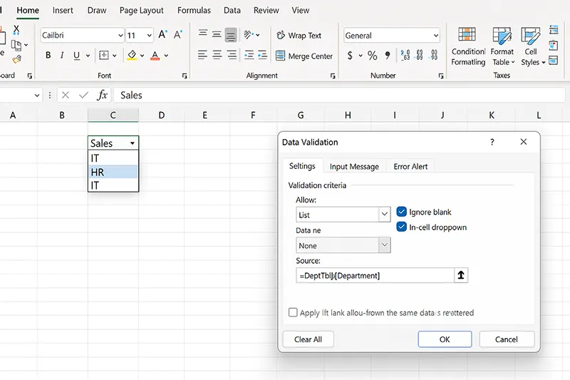
5) Dynamic Drop-Down Lists (Data Validation)

Point Data Validation to a table column so new options appear automatically.

How to do it

1. Create a table (e.g., DeptTbl) with a [Department] column.
2. Select target cells → Data → Data Validation → List.
3. Source: =DeptTbl[Department] → OK.

6) Highlight Overdue Tasks with Conditional Formatting

Make risks visible automatically.

How to do it

1. Select the task range (e.g., rows with Due Date and Status).
2. Home → Conditional Formatting → New Rule → Use a formula.
3. Enter =AND($C2<TODAY(),$D2<>"Done") → choose a red fill → OK.

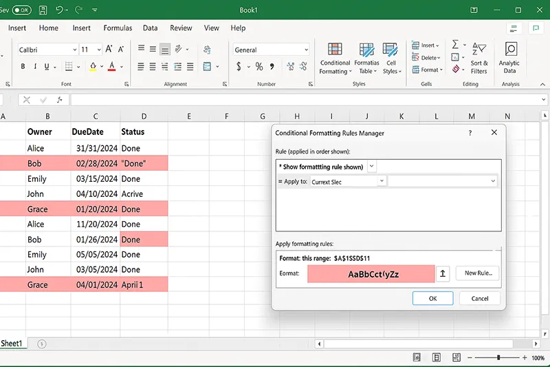
Reference: Microsoft Excel Support

7) Power Query: Clean Data Once, Refresh Forever

Build a repeatable pipeline from CSV, web, or database sources. Click Refresh for next week’s report — no copy-paste.

How to do it

1. Data → Get Data → choose source (CSV/Web/SQL).
2. In Power Query Editor, apply steps (Remove Columns, Split Columns, Change Type, Merge, etc.).
3. Click Close & Load to send to a table or Pivot cache.
4. Next time, just click Refresh All.

8) PivotTables with Slicers (Mini Dashboard)

Interactive summaries for leadership updates — without leaving Excel.

How to do it

1. Select your table → Insert → PivotTable (place on new sheet).
2. Drag fields to Rows/Columns/Values to build metrics.
3. With the Pivot selected: Insert → Slicer → choose filters (Region, Product, Rep).
4. Format slicers (columns, style) and arrange as a mini dashboard.

9) Goal Seek for Break-Even & Targets

Reverse-engineer inputs to hit a result — perfect for pricing and margins.

How to do it

1. Create a cell that calculates the outcome (e.g., Profit).
2. Data → What-If Analysis → Goal Seek.
3. Set Set cell to the outcome, To value to your target, By changing cell to the input (Price/Units).
4. Click OK to solve.

10) LET Function for Cleaner Formulas

Define variables inside a formula and reuse them — easier to read, faster to calculate.

How to do it

1. Structure: =LET(name1,value1,name2,value2,...,calculation_using_names)
2. Example: =LET(qty,[@Qty],price,[@Price],qty*price)
3. Use with IF, LAMBDA, and arrays for complex models.

11) LAMBDA: Build Your Own Function

Package logic once and call it everywhere — no VBA needed.

How to do it

1. Select a blank cell → enter logic using placeholder parameters (e.g., =LAMBDA(x,y, x*y)).
2. Copy the formula → Formulas → Name Manager → New.
3. Name it (e.g., MultiplyXY) and paste the LAMBDA in “Refers to”.
4. Now call =MultiplyXY(5, 6) anywhere.

12) Sparklines for In-Cell Trends

Micro-charts next to rows for quick comparisons.

How to do it

1. Select an output cell → Insert → Line (Sparklines).
2. Set Data Range to the row’s values → OK.
3. Use Sparkline tools to show markers and choose a neutral color.

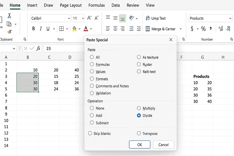
13) Paste Special Power Moves

Paste values, multiply ranges, or transpose in one shot.

How to do it

1. Copy the source cells → right-click destination → Paste Special.
2. Choose Values to strip formulas, Multiply to scale, or Transpose to rotate.
3. Confirm with OK.

14) Go To Special → Fill Blanks

Fix gaps in seconds — great for CRM exports.

How to do it

1. Select the column range → Home → Find & Select → Go To Special → Blanks.
2. Type the value or formula → press Ctrl+Enter to fill all blanks at once.
3. Use =A2 to forward-fill from the cell above.

15) Macro Recorder (Automate Repeated Tasks)

Record once; reuse forever — perfect for formatting and exports.

How to do it

1. View → Macros → Record Macro.
2. Give it a name and (optional) shortcut → perform your steps.
3. Click Stop Recording → run it via Macros list or your shortcut.

Going deeper with automation? See AI in IT Operations.

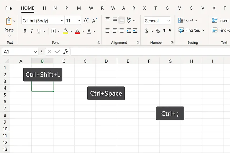
16) Keyboard Shortcuts for Power Users

Compound small wins into minutes saved per task.

How to do it

1. Ctrl+Shift+L — toggle filters.
2. Alt — reveal Ribbon key tips for fast navigation.
3. Ctrl+1 — open Format Cells from anywhere.
4. Ctrl+; / Ctrl+Shift+; — insert today’s date/time.

17) Power Query + Pivot Combo

Excel’s mini ETL + BI flow for SMBs.

How to do it

1. Import and clean with Power Query (Tip 7) → load to a table or the data model.
2. Create a PivotTable on the clean data → add slicers for interactivity.
3. Click Refresh All to update both in one go.

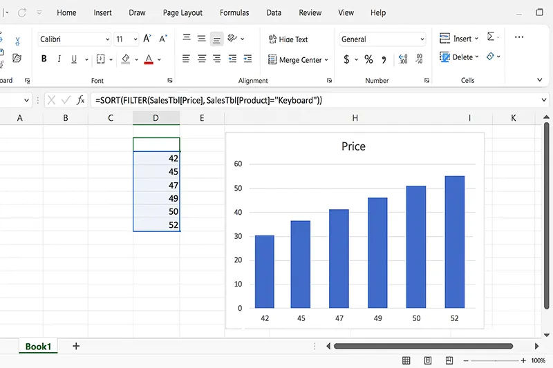
18) Dynamic Arrays as Chart Sources

Live charts that respond to your formulas.

How to do it

1. Build a spilled range with FILTER()/SORT()/UNIQUE().
2. Select the spilled range (include the spill operator if needed, e.g., =A2#).
3. Insert → pick a chart → format axes and labels.

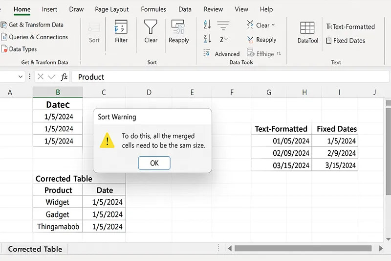
19) Avoid Common Mistakes

• Don’t merge header cells (breaks sorting/filters).
• Don’t mix text and numbers in one column (breaks math/filters).
• Use Data Validation and tables to lock consistency.

How to do it (quick fixes)

1. Unmerge headers → use Center Across Selection if needed.
2. Fix “text-numbers” with Text to Columns or VALUE().
3. Add validation rules for lists, dates, and number ranges.

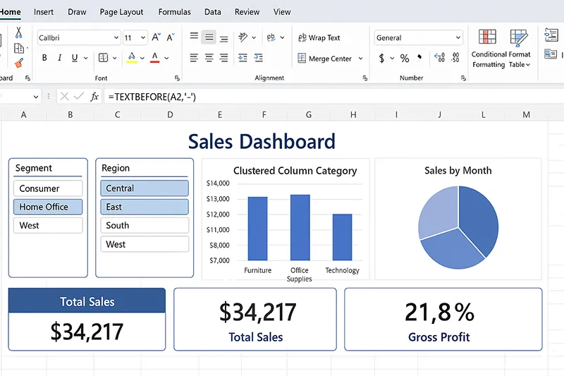
20) Combine Everything into a Dashboard

Pull charts, KPIs, and slicers onto one sheet with a clean theme. It’s a perfect stepping stone to Power BI.

How to do it

1. Create a “Data” sheet (raw), a “Model” sheet (queries/calcs), and a “Dashboard” sheet (visuals).
2. Add PivotCharts and regular charts based on spilled ranges.
3. Add slicers/timelines, align with grid lines, and apply a neutral theme.
4. Test refresh and interaction before sharing.

Final Thoughts

These pro tips aren’t just tricks — they form a practical workflow for modern Excel: structured data, clean formulas, refreshable inputs, and clear visual output. Use tables and dynamic arrays to keep logic stable, Power Query to automate refresh, and dashboards to communicate clearly.

If you’re expanding beyond Excel into collaboration or automation, explore creating Asana portfolios for project dashboards and our guide to AI in IT Operations for process acceleration.