

Overview of the Function
The SUM function adds numbers together and returns the total. It is one of the most commonly used spreadsheet functions and is often the first formula users learn.
You typically use SUM when you need to total sales, expenses, quantities, hours, or any numeric values stored across cells, ranges, or multiple ranges.
The SUM function is fully supported in both Google Sheets and Microsoft Excel. It works in all modern versions of Excel and does not require dynamic array support.
For totals that depend on criteria (for example, “sum only January sales” or “sum only Region A”), use SUMIF instead of SUM.
Key Features and Use Cases
The SUM function solves the problem of manually adding numbers, which is time-consuming and error-prone. It allows you to calculate totals instantly and update results automatically when data changes.
- Add up rows or columns of numbers
- Create totals for reports and dashboards
- Replace manual calculations
- Support analysis and forecasting workflows
Platform Compatibility
- Works in Excel and Google Sheets
- No version limitations
- Supported on desktop, web, and mobile
Sample Data Used in Examples
The first examples use a simple product sales dataset.
Product	Sales
Apples	120
Oranges	95
Bananas	150
Grapes	85
Pears	110
Function Syntax
Syntax
=SUM(number1, [number2], ...)Adds one or more numbers or ranges and returns the total.
Syntax Description
- number1 – The first number, cell, or range to add.
- [number2] – Optional additional numbers, cells, or ranges.
How to Use the Function
If you need to sum only certain rows (for example, only “Apples” or only a specific date range), it’s often better to filter the data first (Google Sheets) or summarize it with a pivot table (Excel), then apply SUM to the results.
- Google Sheets: Use FILTER to return only the rows you want, then SUM the filtered range.
- Excel: Use Pivot Tables to group and total values without writing complex formulas.
How to Use in Google Sheets
Click the cell where you want the total. Type the SUM formula using cell references or ranges, then press Enter. The total updates automatically when values change.
For dynamic subsets (like “only rows where Region = West”), combine SUM with FILTER.
How to Use in Excel
Select the result cell, enter the SUM formula, and press Enter. Excel recalculates totals whenever referenced cells are edited.
If you’re summarizing large datasets, an Excel Pivot Table can often replace multiple SUM formulas.
Examples
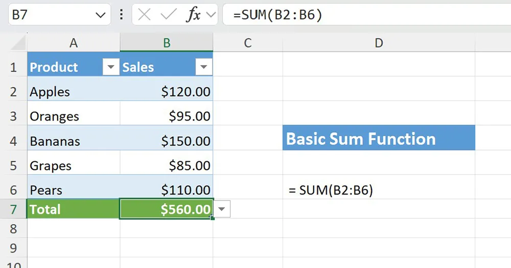
Example 1: Basic Column Total
Platform: Excel and Google Sheets
This example adds all sales values in a single column.
Click cell B7, enter the formula, and press Enter.
=SUM(B2:B6)The formula adds every numeric value in cells B2 through B6.
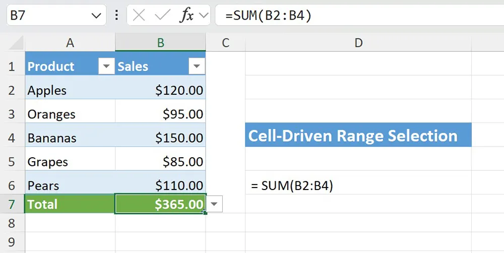
Example 2: Summing a Specific Range
Platform: Excel and Google Sheets
This example totals only part of the data instead of the entire column.
Click cell B8, enter the formula, and press Enter.
=SUM(B2:B4)This approach is useful when you know exactly which rows you want to include. If you want the range to update automatically based on criteria in Google Sheets, filter the rows first with FILTER and then sum the filtered results.
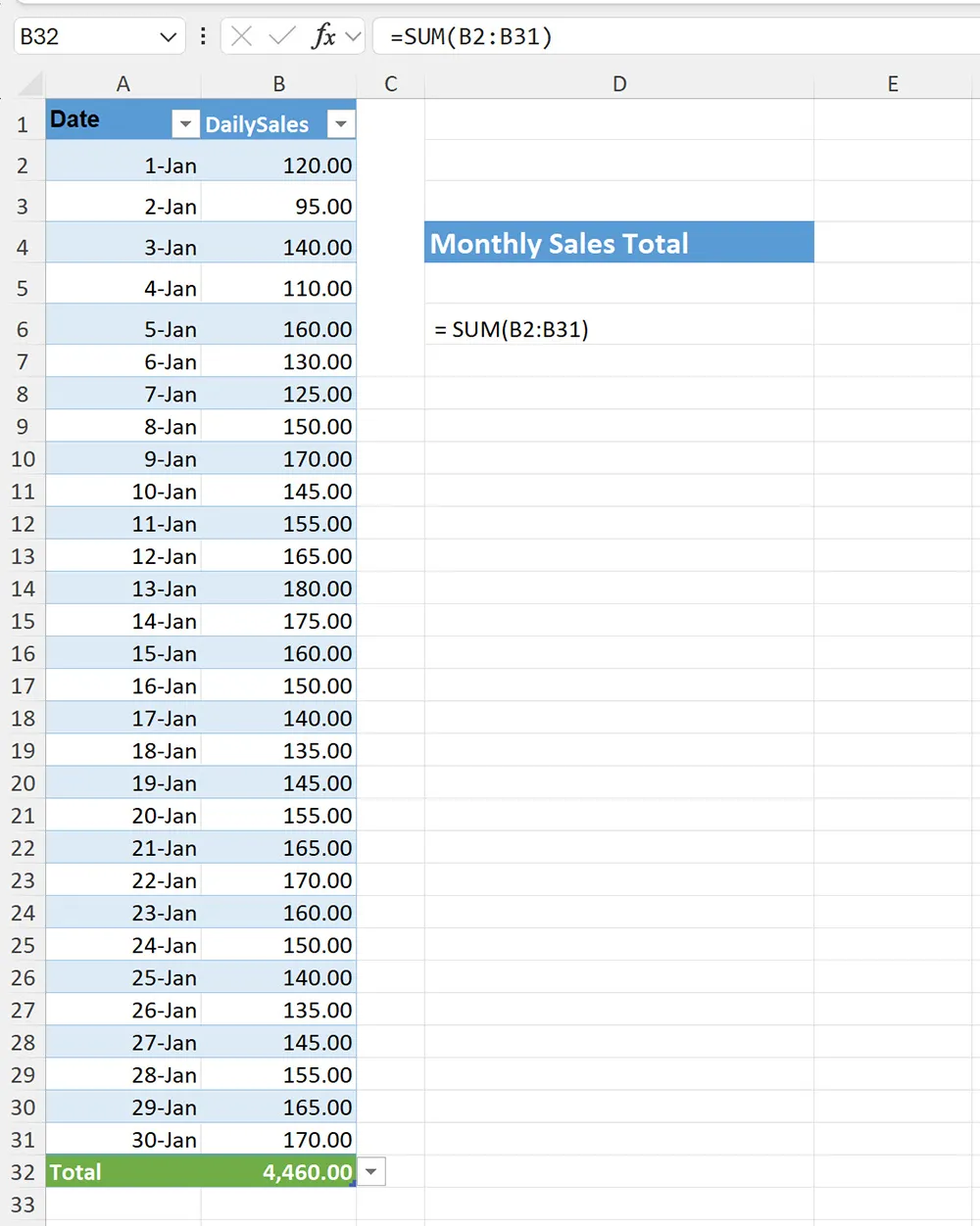
Example 3: Real-World Use Case – Monthly Sales Total
Platform: Excel and Google Sheets
This example calculates total monthly sales from daily sales data.
Date	Daily Sales
Jan 1	120
Jan 2	95
Jan 3	140
Jan 4	110
Jan 5	160
Jan 6	130
Jan 7	125
Jan 8	150
Jan 9	170
Jan 10	145
Jan 11	155
Jan 12	165
Jan 13	180
Jan 14	175
Jan 15	160
Jan 16	150
Jan 17	140
Jan 18	135
Jan 19	145
Jan 20	155
Jan 21	165
Jan 22	170
Jan 23	160
Jan 24	150
Jan 25	140
Jan 26	135
Jan 27	145
Jan 28	155
Jan 29	165
Jan 30	170
Click the total cell below the list (for example, B32), enter the formula, and press Enter.
=SUM(B2:B31)The SUM function aggregates daily values into a single monthly total. If your dataset contains multiple months, create month-based totals by extracting the month with MONTH and grouping month-end dates with EOMONTH. For monthly totals by condition (such as “only online orders”), use SUMIF.
Once you have a monthly total series, you can build projections using FORECAST.
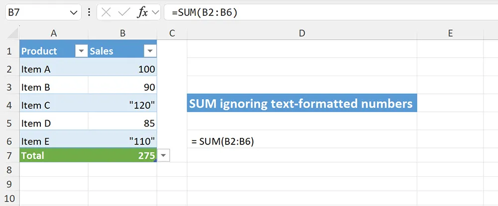
Example 4: Troubleshooting – Ignored Values
Platform: Excel and Google Sheets
This example explains why some values may not be included in a SUM result.
Item	Amount
Item A	100
Item B	90
Item C	"120"
Item D	85
Item E	"110"
Click the result cell (for example, B7), enter the formula, and press Enter.
=SUM(B2:B6)Cells containing text-formatted numbers are ignored. Convert those values to real numbers before summing. If you need to sum only rows that meet a condition (and avoid messy data), filter the dataset first with FILTER (Sheets) or summarize it with Pivot Tables (Excel), then SUM the clean results.
Function vs Alternatives
Use SUM for simple totals.
- SUM vs SUMIF: Use SUMIF when you need totals based on one condition (such as “Region = West”).
- SUM vs FILTER: In Google Sheets, use FILTER to return just the rows you want, then apply SUM to the filtered range.
- SUM vs Pivot Tables: In Excel, Pivot Tables often replace multiple SUM formulas when you need grouped totals (by month, product, or region).
- SUM vs date helpers: Use MONTH and EOMONTH to build month-based groupings before summing.
- SUM vs forecasting: SUM produces totals that are commonly used as inputs for FORECAST when projecting future performance.
Common Errors and Fixes
- Numbers stored as text: Convert values to numeric format so SUM can include them.
- Incorrect ranges: Expand the range to include all rows you intended to add.
- Unexpected totals with filtered lists: SUM still adds hidden rows. In Google Sheets, filter first with FILTER to sum only the visible subset. In Excel, consider a Pivot Table for grouped totals.
- Month-based reporting confusion: If you’re rolling up multiple months, group dates using MONTH or month-end dates using EOMONTH.
Practical Use Cases
- Monthly and yearly financial reports (pair with MONTH and EOMONTH)
- Sales dashboards and KPIs (filter segments with FILTER)
- Grouped totals by category or region (often easier with Pivot Tables)
- Preparing totals for trend projections (use FORECAST)
- Quick validation checks after importing data
Final Thoughts
The SUM function is a foundational tool for spreadsheet analysis. Use it whenever you need reliable totals, and combine it with filtering, month-based grouping, and forecasting functions to build more advanced workflows.
If your totals depend on rules or categories, move from SUM to SUMIF. If you are building monthly reports, pair SUM with MONTH and EOMONTH.