

Dropdown lists are one of the most effective ways to control data entry in Excel. Instead of allowing users to type anything into a cell, you can limit entries to a predefined set of values such as statuses, departments, categories, or approval states. This improves data consistency, reduces cleanup work, and makes reports more reliable.
In 2026, Excel dropdown lists are still built using Data Validation, but the experience differs slightly between Excel for Windows, Excel for macOS, and Excel for the web. The core concepts are the same, but the menus and dialogs look different, which often causes confusion when following older guides.
This tutorial walks through the complete process of creating dropdown lists in Excel, with clear steps for both Windows and macOS users. It also covers how to maintain dropdown lists as your workbook grows, how to prevent common errors, and how to design dropdowns that scale across teams and templates.
What You Will Learn
- How to create a basic dropdown list using Data Validation
- How to build dropdown lists from a cell range, named range, or table
- How Excel dropdown setup differs between Windows and macOS
- How to prevent invalid entries and guide users with messages
- How to troubleshoot broken or inconsistent dropdown behavior
Prerequisites
No prior experience required.
Step-by-Step Instructions
Step 1: Plan and create the source list
Before creating a dropdown, decide where the allowed values should live. While Excel allows inline lists typed directly into Data Validation, this approach becomes difficult to maintain as lists change. A dedicated source list is strongly recommended.
Best practice is to place dropdown values in a single column on the same worksheet or on a separate worksheet named something like Lists or Data. Each value should be in its own cell, with no blank rows in between.
You can copy and paste the following example values directly into Excel to use as a dropdown source list:
Not Started
In Progress
Pending
On Hold
Completed
Cancelled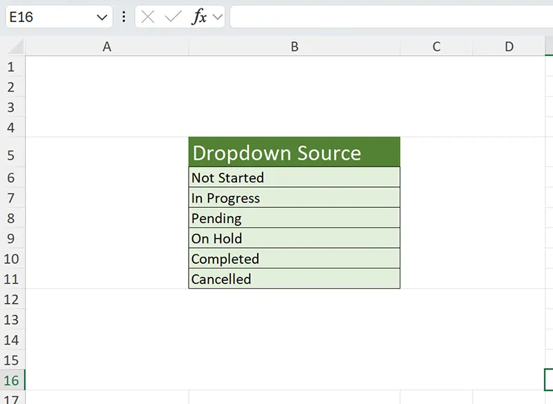
Avoid mixing unrelated lists in the same column. Each dropdown should reference its own clearly defined range to prevent accidental changes later.
Step 2: Select the cell or range for the dropdown
Click the cell where you want the dropdown to appear. If multiple cells need the same dropdown, select the entire range before opening Data Validation. This is especially important if you are working with tables, where new rows should inherit the same validation rules.
If you apply Data Validation to only one cell and later copy it down, incorrect relative references may cause the dropdown source to shift unexpectedly.
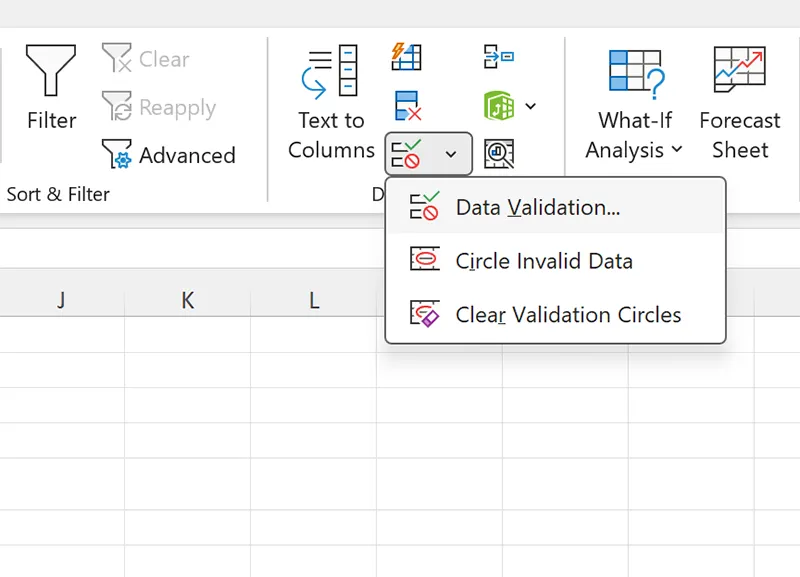
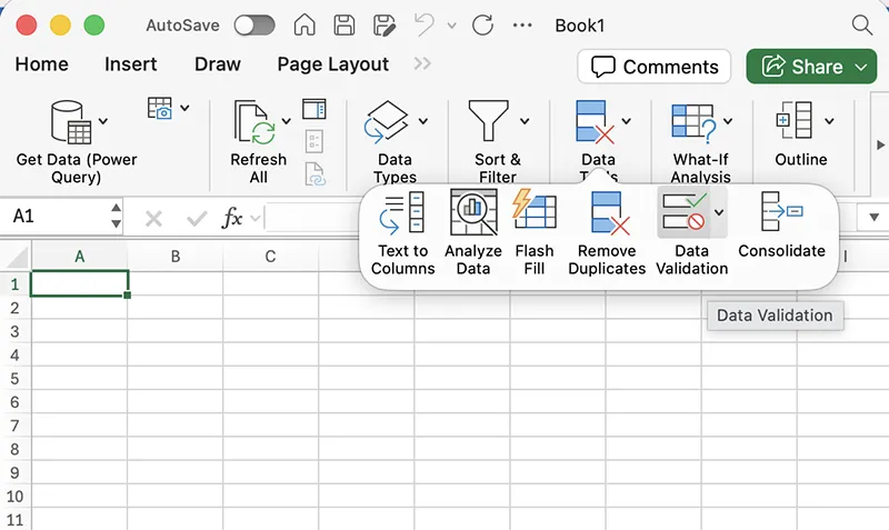
Step 3: Open Data Validation (Windows and macOS)
The Data Validation command is located in the Data tab on both platforms, but the interface looks different.
- Excel for Windows: Data > Data Validation
- Excel for macOS: Data > Data Validation
Step 4: Configure the dropdown list settings
In the Data Validation dialog or pane, configure the following core settings:
- Set Allow to List
- Click into the Source field
- Select the cells containing your source list
- Ensure In-cell dropdown (or In-cell drop-down on macOS) is enabled
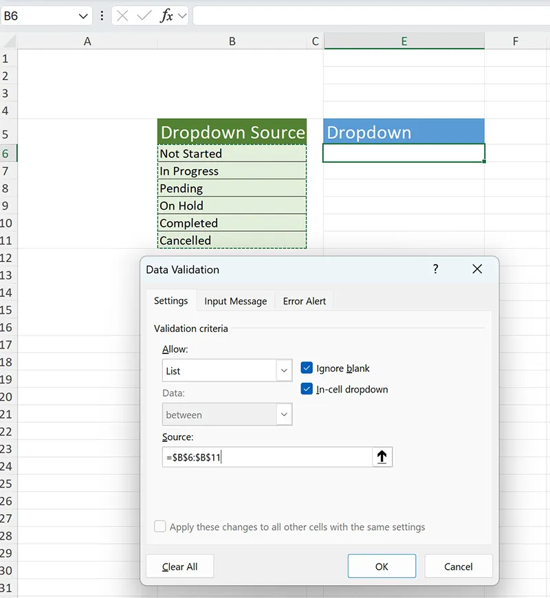
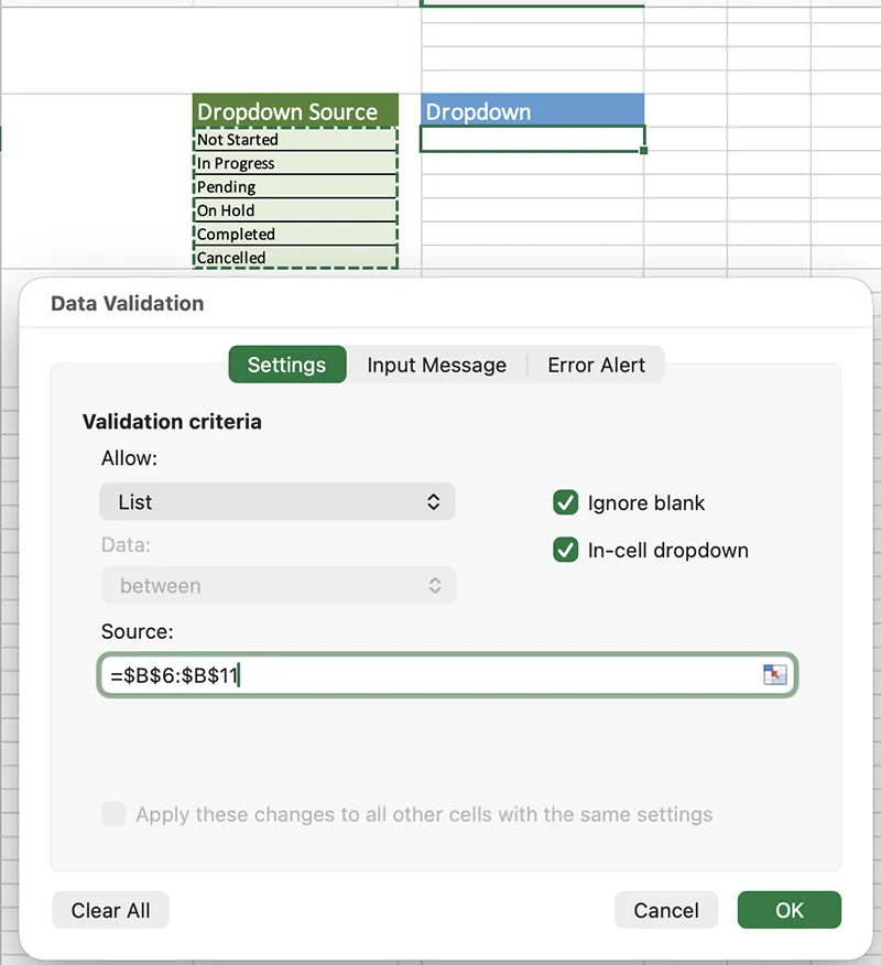
Excel typically converts the selected range into an absolute reference such as =$A$2:$A$6. This is desirable because it prevents the reference from shifting when copied.
Step 5: Control how Excel handles invalid entries
By default, Excel allows users to type values that are not in the dropdown list. To enforce data consistency, configure the Error Alert settings.
- Stop: Blocks invalid entries completely
- Warning: Warns users but allows exceptions
- Information: Displays guidance without enforcement
For most business templates, the Stop option is recommended. Pair it with a clear message such as “Please select a value from the list.”
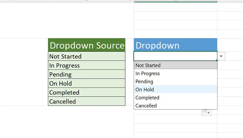
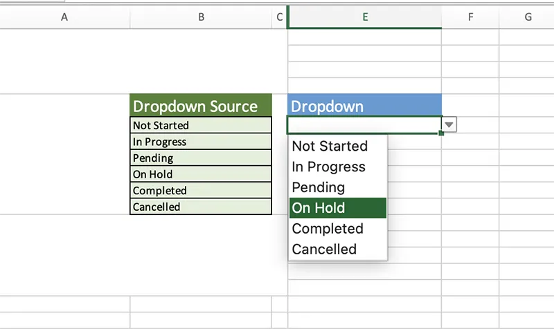
Step 6: Test the dropdown behavior
Click the validated cell and confirm that the dropdown arrow appears. Expand the list and verify that all expected values are present and displayed in the correct order.
Step 7: Make dropdown lists easier to maintain
Range-based dropdowns work, but they require manual updates when new items are added. Two techniques significantly improve long-term maintainability:
- Named ranges: Assign a name to the source list and reference it in Data Validation using
=NameHere. - Excel Tables: Convert the source list to a Table so new entries are automatically included.
Tables are especially effective in shared workbooks because they reduce the risk of broken validation when rows are inserted or deleted.
Common Mistakes and Fixes
- Dropdown arrow is missing: Confirm the cell is not merged and that In-cell dropdown is enabled.
- Blank options appear: Remove blank cells from the source range.
- Validation error appears unexpectedly: The value is not in the list; update the source list if needed.
- Dropdown breaks when copied: Use absolute references or named ranges.
- Different behavior on web vs desktop: Always save the workbook after editing Data Validation in desktop Excel.
Tips and Best Practices
- Keep all dropdown source lists in one dedicated worksheet.
- Use clear, human-readable values rather than abbreviations.
- Lock dropdown cells in protected sheets to prevent accidental changes.
- Apply Data Validation to table columns so new rows inherit rules automatically.
- Document dropdown logic for complex templates used by teams.
Practical Use Cases
- Project status tracking and reporting
- Expense categorization and approvals
- HR onboarding and training tracking
- Academic grading rubrics and evaluations
- Operational dashboards with standardized inputs
Conclusion
Dropdown lists are a foundational Excel feature that dramatically improves data quality with minimal effort. By combining Data Validation with well-structured source lists, named ranges, or tables, you can build spreadsheets that scale cleanly across teams and platforms. Whether you are working on Windows or macOS, the principles remain the same: define trusted values, enforce selection, and design for maintainability.