

SUMIF adds numbers only when a related value meets a condition (called a “criteria”). It’s the go-to function when you need totals like “sum sales for the East region,” “sum hours for a specific employee,” or “sum amounts that are above a threshold.”
If you only need a simple total with no condition, use SUM instead. If you need to return the matching rows (not just a total), see FILTER.
SUMIF works in both Google Sheets and Microsoft Excel. It’s available in modern and older Excel versions, and it does not require dynamic arrays.
Key Features and Use Cases
SUMIF solves the common problem of conditional totals without manual filtering or helper columns. Users typically search for SUMIF when they need quick totals by category, totals above/below a number, or totals within a date rule.
- Replaces manual filtering + adding
- Replaces helper columns that mark rows as “include/exclude”
- Provides fast totals for reports, dashboards, and reconciliations
If you’re browsing related formulas, you can also explore the full functions archive.
Platform Compatibility
- Works in both Excel and Google Sheets: Yes
- Google Sheets only: No
- Excel only: No
Sample Data Used in Examples
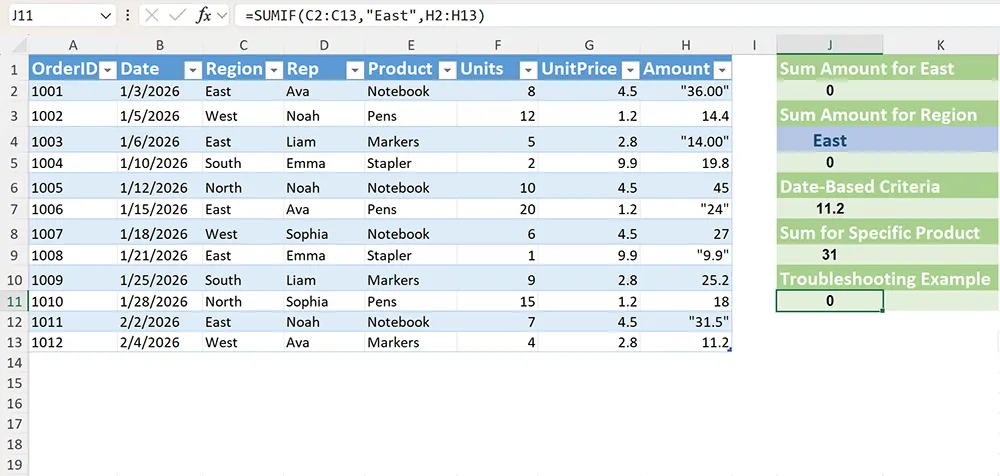
The examples below use a simple sales log with one row per order. You’ll use SUMIF to total amounts based on Region, Rep, and Date criteria.
OrderID	Date	Region	Rep	Product	Units	UnitPrice	Amount
1001	2026-01-03	East	Ava	Notebook	8	4.50	36.00
1002	2026-01-05	West	Noah	Pens	12	1.20	14.40
1003	2026-01-06	East	Liam	Markers	5	2.80	14.00
1004	2026-01-10	South	Emma	Stapler	2	9.90	19.80
1005	2026-01-12	North	Noah	Notebook	10	4.50	45.00
1006	2026-01-15	East	Ava	Pens	20	1.20	24.00
1007	2026-01-18	West	Sophia	Notebook	6	4.50	27.00
1008	2026-01-21	East	Emma	Stapler	1	9.90	9.90
1009	2026-01-25	South	Liam	Markers	9	2.80	25.20
1010	2026-01-28	North	Sophia	Pens	15	1.20	18.00
1011	2026-02-02	East	Noah	Notebook	7	4.50	31.50
1012	2026-02-04	West	Ava	Markers	4	2.80	11.20
Function Syntax
Syntax
=SUMIF(range, criteria, [sum_range])Syntax Short Description
Sums values that meet a single condition.
Syntax Description
-
range: The cells to test against your condition (text, numbers, dates, or logical values).
-
criteria: The condition that decides which rows to include (for example: “East”, “>=100”, “>=”&DATE(2026,2,1)).
-
[sum_range] (optional): The cells to add. If omitted, SUMIF sums the cells in range when they meet the criteria.
How to Use in Google Sheets
-
Click the cell where you want the total to appear.
-
Type your SUMIF formula (start with =).
-
Press Enter. Google Sheets calculates the conditional total and shows the result.
How to Use in Excel
-
Click the cell where you want the total to appear.
-
Type your SUMIF formula (start with =), or select Formulas > Insert Function and search for SUMIF.
-
Press Enter. Excel returns a single value (SUMIF does not spill).
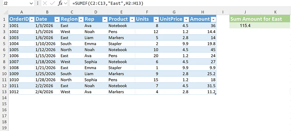
Example 1: Basic SUMIF by Text Criteria (Sum Amount for East)
Platform: Excel and Google Sheets
Scenario: You want the total Amount for orders in the East region.
-
Click cell J2.
-
Enter the formula below and press Enter.
-
Expected result: The sum of Amount values where Region is East.
=SUMIF(C2:C13,"East",H2:H13)How it works: SUMIF checks each cell in C2:C13 (Region). When it equals “East”, it adds the corresponding value from H2:H13 (Amount) to the total.
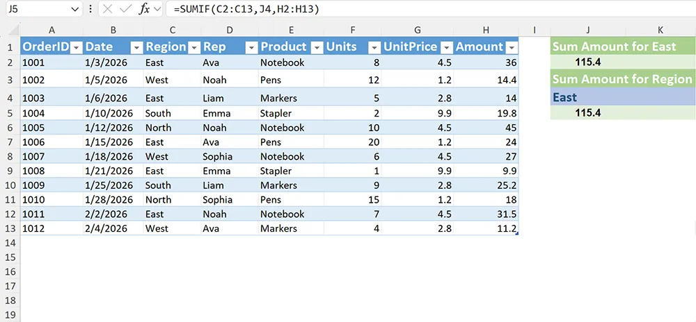
Example 2: Cell-Driven Criteria (Sum Amount for the Region in J4)
Platform: Excel and Google Sheets
Scenario: You want the total to change automatically when a user selects a different region.
-
Type a region name (for example, East or West) into cell J4.
-
Click cell J5.
-
Enter the formula below and press Enter.
-
Expected result: A total that updates whenever J4 changes.
=SUMIF(C2:C13,J4,H2:H13)How it works: The criteria comes from J4, so the formula recalculates based on whatever text is in that cell.
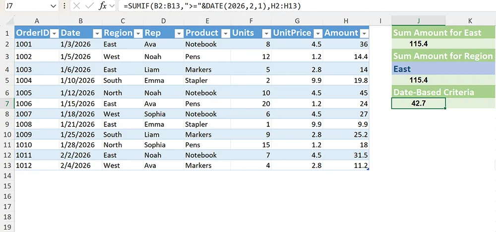
Example 3: Date-Based Criteria (Sum Amount on or After 2026-02-01)
Platform: Excel and Google Sheets
Scenario: You want to sum Amount for orders on or after a specific date.
-
Click cell J7.
-
Enter the formula below and press Enter.
-
Expected result: A total of Amount for rows where Date is on/after 2026-02-01.
=SUMIF(B2:B13,">="&DATE(2026,2,1),H2:H13)How it works: SUMIF tests the Date column (B2:B13) against a criteria string. The >= operator is combined with a real date value created by DATE(2026,2,1).
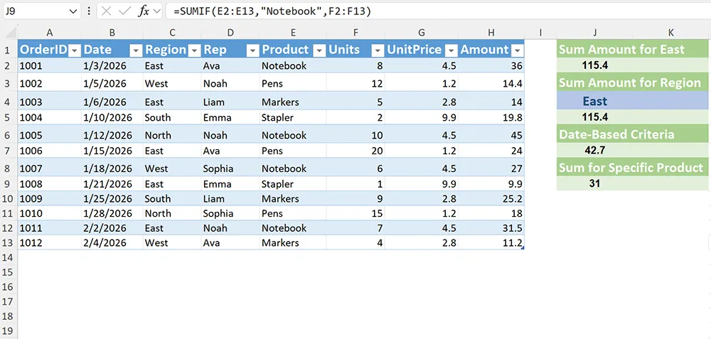
Example 4: Practical Real-World Use Case (Sum Units for a Specific Product)
Platform: Excel and Google Sheets
Scenario: You want to total the Units sold for one product (for example, Notebook) to support inventory planning.
-
Click cell J9.
-
Enter the formula below and press Enter.
-
Expected result: Total Units where Product equals “Notebook”.
=SUMIF(E2:E13,"Notebook",F2:F13)How it works: SUMIF checks the Product column (E2:E13) for “Notebook” and adds the matching Units from F2:F13.
Example 5: Troubleshooting Example (SUMIF Returns 0 Because Amount Is Stored as Text)
Platform: Excel and Google Sheets
Scenario: Your SUMIF formula looks correct, but it returns 0 or a smaller number than expected. A common cause is that the values in the sum range are stored as text.
-
Click cell J11 and enter a typical SUMIF (example below).
-
If the result is wrong, confirm whether Amount values are text (often left-aligned, or include hidden characters).
-
Fix by converting the sum range to numbers, then recalculate.
=SUMIF(C2:C13,"East",H2:H13)How it works (and why it fails): SUMIF can only add numeric values. If H2:H13 contains text like “36.00” instead of the number 36, SUMIF may treat those cells as 0.
Fix options:
-
Google Sheets: Select H2:H13 > Format > Number, then use Data > Data cleanup options if needed.
-
Excel: Select H2:H13 > use the warning icon (if shown) to Convert to Number, or use Data > Text to Columns > Finish.
Function vs Alternatives
Use SUMIF when you have a single condition to test. If you need more than one condition (for example, Region = East AND Rep = Ava), use SUMIFS instead.
-
SUMIF: One condition; fastest and simplest for single-criteria totals.
-
SUMIFS: Multiple conditions (AND logic by default); best for multi-filter totals.
-
Lookup functions: Return a value from one matching row; not meant for summing multiple matches.
-
Helper columns: Useful in older workflows, but SUMIF usually replaces “flag then sum” approaches.
-
Pivot tables: Great for interactive summaries and multiple totals, but heavier than a single formula.
-
When you need the matching rows (not a total): Use FILTER to return only the rows that meet your condition.
-
When you need a simple total with no condition: Use SUM.
Common Errors and Fixes
-
SUMIF returns 0: The criteria doesn’t match the data exactly (extra spaces, different spelling, hidden characters).
Fix: Clean the criteria range (TRIM/CLEAN) or standardize values with data validation.
-
SUMIF returns a smaller total than expected: The sum range contains text numbers.
Fix: Convert the sum range to numbers (format and conversion tools), then recalculate.
-
Criteria operators not working: You wrote something like >=A1 without concatenation.
Fix: Build operator criteria with concatenation, like “>=”&A1.
-
Wrong totals due to mismatched ranges: The criteria range and sum range are different sizes.
Fix: Ensure range and sum_range cover the same number of rows.
Practical Use Cases
-
Sales dashboards: total revenue by region, rep, or product
-
Operations tracking: total units shipped for a SKU
-
Budgeting: total spend by category (travel, supplies, software)
-
Time tracking: total hours by employee or project code
-
Data cleanup checks: sum values that exceed thresholds to spot outliers
If you’re building broader analysis workflows, you may also use conditional totals alongside forecasting (see FORECAST) when projecting future values from historical results.
Conclusion
Use SUMIF when you need a conditional total based on one rule. Keep the ranges aligned, build operator-based criteria with concatenation, and verify your sum range contains real numbers.
A helpful mental model: SUMIF is “filter by one condition, then add the matching values.” If you need more than one condition, step up to SUMIFS.