FILTER Function in Excel & Google Sheets (Syntax + Examples + Fixes)

Overview

If you want a fast way to pull the exact rows you need from a larger dataset, the FILTER function is one of the most useful tools in Google Sheets and modern Excel. It returns only the rows that meet your criteria, and it updates automatically when the source data changes. This guide is written for beginners who want quick wins, plus intermediate users who need reliable patterns for multiple conditions, date filtering, and troubleshooting.

Platform support matters: Google Sheets supports FILTER natively. Excel supports FILTER in Microsoft 365 and Excel 2021+ (dynamic arrays). If you are using an older Excel version, you may need alternative approaches such as Advanced Filter, Power Query, or helper columns.

At a glance:

• Google Sheets: Supported
• Excel: Supported in Microsoft 365 and Excel 2021+ (dynamic arrays required)
• What it does: Returns a filtered range of data based on one or more conditions, updating results automatically

Key Features and Sections

People usually search FILTER because they want to do one of these tasks quickly:

• Filter rows where a column equals a value (for example, Region = West)
• Apply multiple conditions (AND / OR logic)
• Filter by dates (last 30 days, between two dates)
• Fix errors such as no matches, mismatched ranges, or text-vs-number issues
• Decide whether FILTER is better than VLOOKUP/XLOOKUP, QUERY, or Advanced Filter

This article follows that exact intent flow: definition, syntax, the most common example, advanced patterns, differences between Excel and Google Sheets, fixes for common problems, and practical ways to use FILTER in real work.

Platform Compatibility for This Post

All FILTER formulas shown in Examples 1–6 work in both Google Sheets and Excel (Microsoft 365 / Excel 2021+), unless a note explicitly says “Google Sheets only” or “Excel only.”

• Works in both: FILTER, TODAY, basic comparisons (=, >, >=, <=), AND/OR logic using * and +
• Google Sheets only (optional comparison later): QUERY, ARRAYFORMULA
• Excel only (optional enhancement later): Structured references with Excel Tables

Sheet1: Sample Sales Data

Use the following sample dataset to follow along in either Excel or Google Sheets. Paste it into cell A1. It is tab-delimited (so it lands in columns correctly).

Date	Region	Department	Sales	Rep	Status
2026-01-03	West	IT	1450	Ayesha	Open
2026-01-05	East	HR	820	Liam	Closed
2026-01-06	North	Sales	2100	Noah	Open
2026-01-08	West	Marketing	640	Sophia	Open
2026-01-09	South	IT	1200	Ethan	Closed
2026-01-10	West	Sales	980	Olivia	Open
2026-01-12	East	Finance	1750	Mason	Open
2026-01-14	North	HR	430	Amelia	Closed
2026-01-15	West	IT	2600	James	Open
2026-01-17	South	Sales	1500	Isabella	Open
2026-01-18	East	Marketing	700	Benjamin	Closed
2026-01-20	West	Finance	1100	Mia	Open
2026-01-21	North	IT	900	Lucas	Open
2026-01-22	South	HR	1050	Charlotte	Open
2026-01-23	East	Sales	1990	Henry	Open
2026-01-24	West	Marketing	1300	Evelyn	Closed
2026-01-25	North	Finance	1600	Alexander	Open
2026-01-26	South	IT	300	Abigail	Closed
2026-01-27	West	Sales	2400	Daniel	Open
2026-01-28	East	HR	980	Emily	Open
2026-01-29	West	IT	750	Matthew	Open
2026-01-30	North	Marketing	1250	Harper	Closed

Tip for Excel users: place your FILTER formula in an empty area with enough space below and to the right for results to spill.

How to Use the Template

FILTER is easy to learn because the core idea is always the same: provide the range you want to return, then provide a condition range that evaluates to TRUE/FALSE for each row. If your include test returns TRUE for a row, that row is returned in the output.

A reliable workflow is to keep your raw data in one place and create filtered “views” in separate areas or separate worksheets. This reduces manual filtering and makes your reports more consistent for teams.

How to Use FILTER in Google Sheets

• 1) Paste your data into a clean range with headers (for example, A1:F31).
• 2) Click an empty cell where you want the filtered results to appear (for example, H2).
• 3) Type a FILTER formula using the range you want returned and the criteria range that should be TRUE.
• 4) Press Enter. The filtered results will expand automatically.
• 5) If you see no results, add an if_empty message so it is clear the formula ran successfully.

How to Use FILTER in Excel (Microsoft 365 / Excel 2021+)

• 1) Confirm your Excel version supports dynamic arrays (Microsoft 365 or Excel 2021+).
• 2) Paste your data into a consistent range with headers (for example, A1:F31).
• 3) Choose an output cell with enough empty space for results to spill (for example, H2).
• 4) Enter the FILTER formula and press Enter.
• 5) If results do not show, clear any cells blocking the spill range.

FILTER Function Syntax (Excel vs Google Sheets)

Works in: Google Sheets and Excel (Microsoft 365 / Excel 2021+).

=FILTER(array, include, if_empty)

• array: The range of data you want returned (for example, A1:F31)
• include: One or more TRUE/FALSE tests that match the number of rows in the array
• if_empty: Optional text to show if no results match (recommended)

Practical note: The include range must align row-for-row with the array. If your array is A2:F31, your include test should also be built from ranges that start at row 2 and end at row 31.

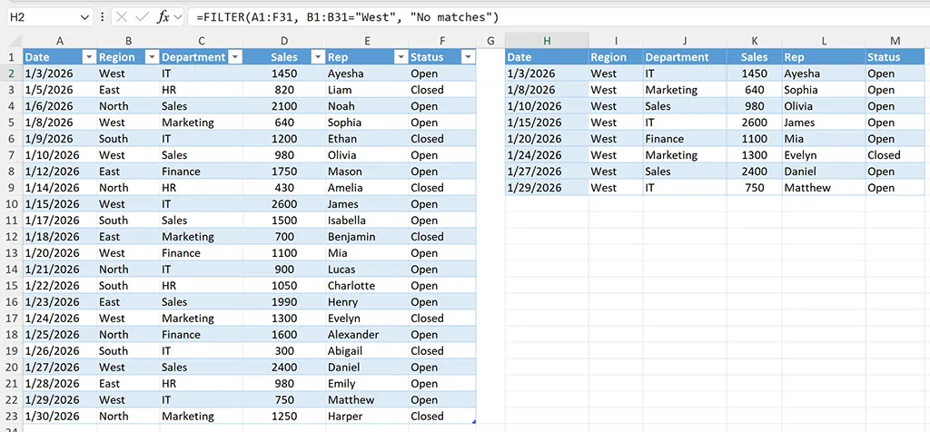
Example 1: Basic FILTER (Most Common Search Intent)

Works in: Google Sheets and Excel (Microsoft 365 / Excel 2021+).

Scenario: Filter sales data where Region = “West”. This is the best first example because it mirrors the most common real-world question: “Show me only the West rows.”

Steps:

• 1) In Google Sheets, click H2.
• 2) Enter: =FILTER(A1:F31, B1:B31=”West”, “No matches”)
• 3) Press Enter.

=FILTER(A1:F31, B1:B31="West", "No matches")

How it works:

• A1:F31 is the data returned (multiple columns)
• B1:B31=”West” creates a TRUE/FALSE list for each row
• if_empty displays a friendly message when no rows match

Example 2: FILTER with Multiple Conditions (AND)

Works in: Google Sheets and Excel (Microsoft 365 / Excel 2021+).

Multiple conditions are a top search use case because they replace helper-column workflows. For AND logic, multiply conditions using * so both tests must be TRUE.

Steps:

• 1) Clear the previous output area.
• 2) In H5, enter the AND formula: =FILTER(A1:F31, (B1:B31=”West”)*(D1:D31>1000), “No matches”)

=FILTER(A1:F31, (B1:B31="West")*(D1:D31>1000), "No matches")

Why this pattern is reliable:

• Each condition is wrapped in parentheses, which reduces logic mistakes
• The include test remains aligned with the returned array (row-for-row)
• You can extend the AND chain by multiplying additional conditions

Example 3: FILTER with Multiple Conditions (OR)

Works in: Google Sheets and Excel (Microsoft 365 / Excel 2021+).

For OR logic, add conditions using + so either test can be TRUE. This is useful for cases like “IT or HR,” “Open or Pending,” or “East or West.”

Steps:

• 3) Put the OR example below it (for example in H14): =FILTER(A1:F31, (C1:C31=”IT”)+(C1:C31=”HR”), “No matches”)

=FILTER(A1:F31, (C1:C31="IT")+(C1:C31="HR"), "No matches")

Common mistake to avoid: If your text values have extra spaces (for example, “IT ” instead of “IT”), OR logic can appear “broken.” If results look wrong, check for inconsistent text formatting in the source data.

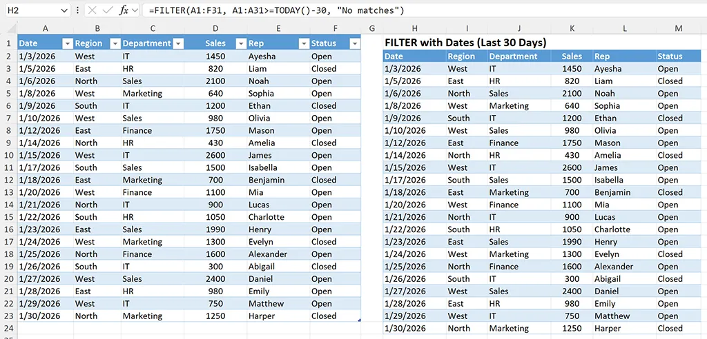
Example 4: FILTER with Dates (Last 30 Days)

Works in: Google Sheets and Excel (Microsoft 365 / Excel 2021+).

Date filtering is extremely popular for operational reports, but it is also a common failure point when dates are stored as text. This example returns rows from the last 30 days using TODAY().

Steps:

• 1) Click H2.
• 2) Enter: =FILTER(A1:F31, A1:A31>=TODAY()-30, “No matches”)

=FILTER(A1:F31, A1:A31>=TODAY()-30, "No matches")

Why date filtering can fail (and how to avoid it):

• If dates do not sort correctly, they may be text. Convert them to real dates before filtering.
• Imported CSVs can introduce mixed date formats; standardize the Date column first.
• Be consistent with locale formatting so month/day does not swap unexpectedly.

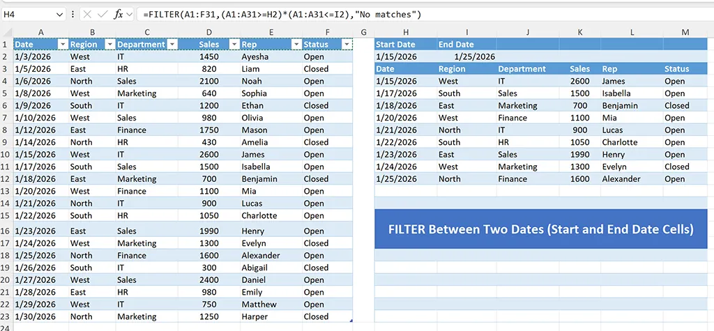
Example 5: FILTER Between Two Dates (Start and End Date Cells)

Works in: Google Sheets and Excel (Microsoft 365 / Excel 2021+).

This date example is easy to reuse because the criteria is visible in cells. Put a start date in G2 and an end date in H2, then filter rows between those dates.

Steps (Excel):

• 1) In Excel, create criteria cells: H1: Start Date, I1: End Date, H2: 2026-01-15, I2: 2026-01-25
• 2) Click H4 and enter: =FILTER(A1:F31,(A1:A31>=H2)*(A1:A31<=I2),”No matches”)

=FILTER(A1:F31,(A1:A31>=H2)*(A1:A31<=I2),"No matches")

Best practice: Label your criteria cells (for example, “Start Date” and “End Date”) so it is clear which inputs drive the results.

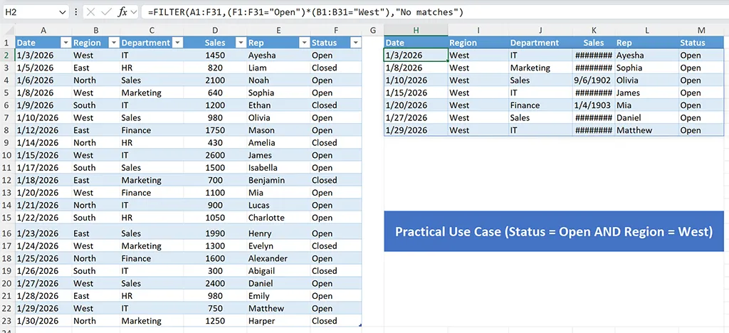
Example 6: Practical Use Case (Status = Open AND Region = West)

Works in: Google Sheets and Excel (Microsoft 365 / Excel 2021+).

This is a realistic dashboard pattern used for “Open items,” “Active tickets,” or “Current tasks.” It returns only records where Status is Open and Region is West.

Steps (Excel):

• 1) In Excel, click H2 (or a clean output cell).
• 2) Enter: =FILTER(A1:F31,(F1:F31=”Open”)*(B1:B31=”West”),”No matches”)
• 3) Make sure Region and Status columns are visible in the source.

=FILTER(A1:F31,(F1:F31="Open")*(B1:B31="West"),"No matches")

Tip for dashboards: Place this output on a separate “Dashboard” or “Summary” worksheet and keep the raw data on “Data.” That separation reduces accidental edits and makes the workbook easier to share.

Example 7: Filter Mismatched Range

Create a controlled “wrong formula” example to understand what a range mismatch looks like.

Steps:

• 1) Click H2.
• 2) Enter a mismatched-range formula like: =FILTER(A1:F31, B1:B10=”West”, “No matches”)
• 3) The mismatch should trigger an error.

=FILTER(A1:F31, B1:B10="West", "No matches")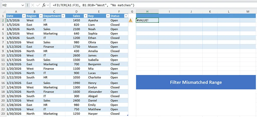

FILTER vs Traditional Alternatives (Decision-Based Intent)

FILTER is not a replacement for every data task. It is best when you want to return rows that match conditions and keep results live. Use these quick comparisons to choose the right tool.

• FILTER vs VLOOKUP/XLOOKUP: FILTER returns many rows; lookup functions usually return one matching value per row.
• FILTER vs QUERY (Google Sheets): QUERY is powerful for SQL-like grouping and selection; FILTER is simpler for straightforward conditions.
• FILTER vs Advanced Filter (Excel): Advanced Filter is useful for one-time extraction; FILTER is dynamic and updates automatically.
• FILTER vs helper columns: FILTER often eliminates helper columns, reducing sheet complexity and maintenance.

Decision tip: If your output should change the moment new rows are added, FILTER is usually the right starting point.

Google Sheets Only: QUERY Comparison (Optional)

Works in: Google Sheets only. Not available in Excel.

If you use Google Sheets, QUERY is often compared to FILTER. QUERY is excellent when you want SQL-like selection and you are comfortable with query strings. FILTER is usually easier to learn and easier to audit.

=QUERY(A1:F31, "select * where B = 'West'", 1)

Excel Only: Structured References with Tables (Optional)

Works in: Excel only (when your data is in an Excel Table). Google Sheets does not use structured references in the same way.

If you convert your data range to an Excel Table (Insert > Table), you can use table references for cleaner formulas. The logic is the same, but the references are easier to maintain when the table grows.

=FILTER(Table1, Table1[Region]="West", "No matches")

Excel vs Google Sheets Differences (Trust Builder)

Most FILTER behavior is similar, but a few differences matter in daily use:

• Excel version requirement: FILTER works in Microsoft 365 and Excel 2021+. If you do not have dynamic arrays, you will not have FILTER.
• Spill behavior (Excel): Results spill into adjacent cells. If any cell in the spill range is not empty, Excel returns a spill-related error and no results display.
• Performance: Very large ranges can slow recalculation in both platforms. Restrict ranges to realistic bounds instead of entire columns when possible.
• Google Sheets recalculation: In shared spreadsheets, results can recalculate more frequently. Keep ranges tight for performance.

Why Choose This Template

A repeatable FILTER approach is valuable because it turns messy, manual filtering into a consistent workflow you can reuse across reports. When your team relies on the same workbook or shared spreadsheet, consistency reduces errors and makes troubleshooting faster.

Practical benefits you can expect from a well-built FILTER setup:

• Cleaner dashboards: Pull only the rows you need into a summary view.
• Live reporting: As new transactions are added, your filtered output updates automatically.
• Fewer manual steps: No repeated clicking of filter dropdowns and no copying/pasting filtered results.
• Lower risk of mistakes: Conditions live in formulas where they can be reviewed and standardized.

Common FILTER Errors and Fixes

When FILTER “doesn’t work,” it is usually one of these issues. Use this checklist to fix problems quickly.

Mismatched Range Sizes

Symptom: Error or unexpected results. Cause: Your array range and include range do not have the same number of rows.

• Fix: If your array is A2:F31, your include range must be something like B2:B31 or D2:D31, not B2:B200 or B:B.

No Results Returned

Symptom: Error or blank output. Cause: Nothing matches the criteria.

• Fix: Add an if_empty message so it is clear the formula is working.
• Fix: Check for extra spaces and inconsistent casing in imported text values (for example, “West ” vs “West”).

Text vs Number Comparisons

Symptom: A numeric condition like Sales > 1000 returns no matches. Cause: Numbers are stored as text (often after imports).

• Fix: Convert the column to real numbers using your platform’s conversion options before filtering.
• Fix: Watch for currency symbols and commas that force text formatting.

Date Criteria Not Matching

Symptom: Date filters return incorrect or zero rows. Cause: Dates are stored as text or mixed formats.

• Fix: Confirm dates sort oldest-to-newest correctly; incorrect sorting often indicates text dates.
• Fix: Standardize date imports and avoid mixing locale formats in the same column.

Excel Spill Blocked

Symptom: In Excel, FILTER returns a spill-related error and no results display. Cause: Cells in the output spill range are not empty.

• Fix: Clear the cells where the results would spill, or move the formula to an area with enough space.

Practical Use Cases

FILTER becomes significantly more valuable once you apply it to real workflows. Here are practical ways teams use it in Excel and Google Sheets.

• Dynamic dashboards: Filter a dataset by region, owner, or status, then summarize the filtered results elsewhere.
• Live operational reports: Show “today’s items,” “this week’s tickets,” or “open requests” based on date and status criteria.
• Attendance and scheduling: Filter by date range and team to produce a current roster view.
• Sales pipelines: Filter deals by stage, probability, or rep, and keep a live view for weekly reviews.
• Audit and cleanup: Filter rows where required fields are blank or where values exceed thresholds.

Best practice: Keep your source data as a clean table (consistent headers, one record per row), then build FILTER-based views for each audience. This is easier to secure and easier to maintain than copying subsets into separate files.

In a Nutshell:

The FILTER function is one of the fastest ways to create live, condition-based views of your data in Google Sheets and modern Excel. Start with a simple “equals” condition, then build up to multiple conditions and date filtering using consistent, aligned ranges. When something goes wrong, the fix is usually straightforward: check range alignment, confirm data types (numbers and dates), add an if_empty message, and make sure your output area is clear for spill results in Excel.